
Using Python Multiprocessing with NLLS Regression
In my previous article, I looked at some of the modules available for Nonlinear Least Squares (NLLS) Regression in Python. I also tested and discussed various options among these modules including the choice of fitting algorithms and whether an explicit Jacobian is provided, and looked at the speed differences among these options. Continuing with this theme of improving the speed of running NLLS Regression fitting on a set of data, in this article, I will look at possible speed improvements from parallel computing. That is, if we are doing repeated jobs over and over, is it possible to divide up the work such that we can execute computations in parallel to reduce the total time it takes to run our job/script? Often in low-level languages such as C/C++, this is often accomplished using multithreading. In multithreading, computing code can be broken up into smaller snippets of code called threads, which can run concurrently and pass memory back and forth. For the Python language, this is actively discouraged by design.
From the Python documentation: "In CPython, due to the Global Interpreter Lock (GIL), only one thread can execute Python code at once (even though certain performance-oriented libraries might overcome this limitation). If you want your application to make better use of the computational resources of multi-core machines, you are advised to use multiprocessing or concurrent.futures.ProcessPoolExecutor. However, threading is still an appropriate model if you want to run multiple I/O-bound tasks simultaneously." Since regression fitting algorithms' performance deals mostly with computing speed and not I/O issues, we'll take a look at the suggestion from the documentation - the Python multiprocessing module.
What Is Multiprocessing and What Can it Do?
A process is an instance of a computing program running on a computer. Each process is encapsulated by itself on the operating system, and each process can be made up of multiple threads. Thus, multithreading attempts to speed up computing time by dividing code up into multiple threads within the same process. Of course, explicit multithreading has its drawbacks, with issues such as race conditions or deadlocks. As noted in the Python documentation on the GIL: “This simplifies the CPython implementation by making the object model (including critical built-in types such as dict) implicitly safe against concurrent access. Locking the entire interpreter makes it easier for the interpreter to be multi-threaded, at the expense of much of the parallelism afforded by multi-processor machines.” So, it seems the Python language focuses on safety of memory access and simplicity of execution at the expense of speed improvements that could be made in a lower-level language. Note, that Python (CPython) is built on top of the C language, which can be multithreaded. Allowing Python to be multithreaded on top of the inner workings of the Python code written in C could lead to multiple layers of multithreading, which might be fun...
One specific note before we dive into Python’s multiprocessing module - safety of memory access is an important concept for a process running on a modern operating system. One process running on a computer is NOT allowed to access memory on a different process (unless explicitly defined). When one process attempts to access another processes’ memory, this results in a memory access violation or segmentation fault (segfault for short). When this happens, most operating systems will kill the violating process, causing the program to abruptly terminate (aka crash). This is by design – think of how hard it would be to debug your program if another program/process on your machine was changing your program’s memory. Alternatively, if your program decrypted some data and was processing it in memory, malware running on your computer could access this decrypted data. While one process can’t access other memory in wantonly ways, a process is allowed to access another process’s memory in explicitly defined ways for each operating system. Using these communication methods such as pipes comes with a performance hit on the overhead of using such methods, but in our case, we hope executing code in parallel will be worth it.
Let’s take a look at how the Python process runs on my local PC running Windows 10. I will again be running this test in Visual Studio Code, so first I opened VS Code open and then opened the Python script I created for this article. If I open up Task Manager on Windows (keyboard shortcut: Ctrl+Shift+Esc), make sure the “Processes” tab is selected, and under the “Apps” section, click on the arrow next to “Visual Studio Code”, I will get a list of all processes currently running under VS Code, which should include one or more Python processes. The number on your machine may vary based on what toolkits you have installed on VS Code, how many scripts are open, whether you have a code linter installed, etc. The following image shows you what appears in Task Manager on my machine:

We can learn even more about our Python processes if we select the “Performance” tab in Task Manager, and down near the bottom, there should be a link that says “Open Resource Monitor”. The Resource Monitor allows you to see more detail about what process are running on what CPU cores, and how much memory and disk space they are using, among other things. Here is a snapshot I took on my machine with the two Python processes running on VS Code focused on in the process list:
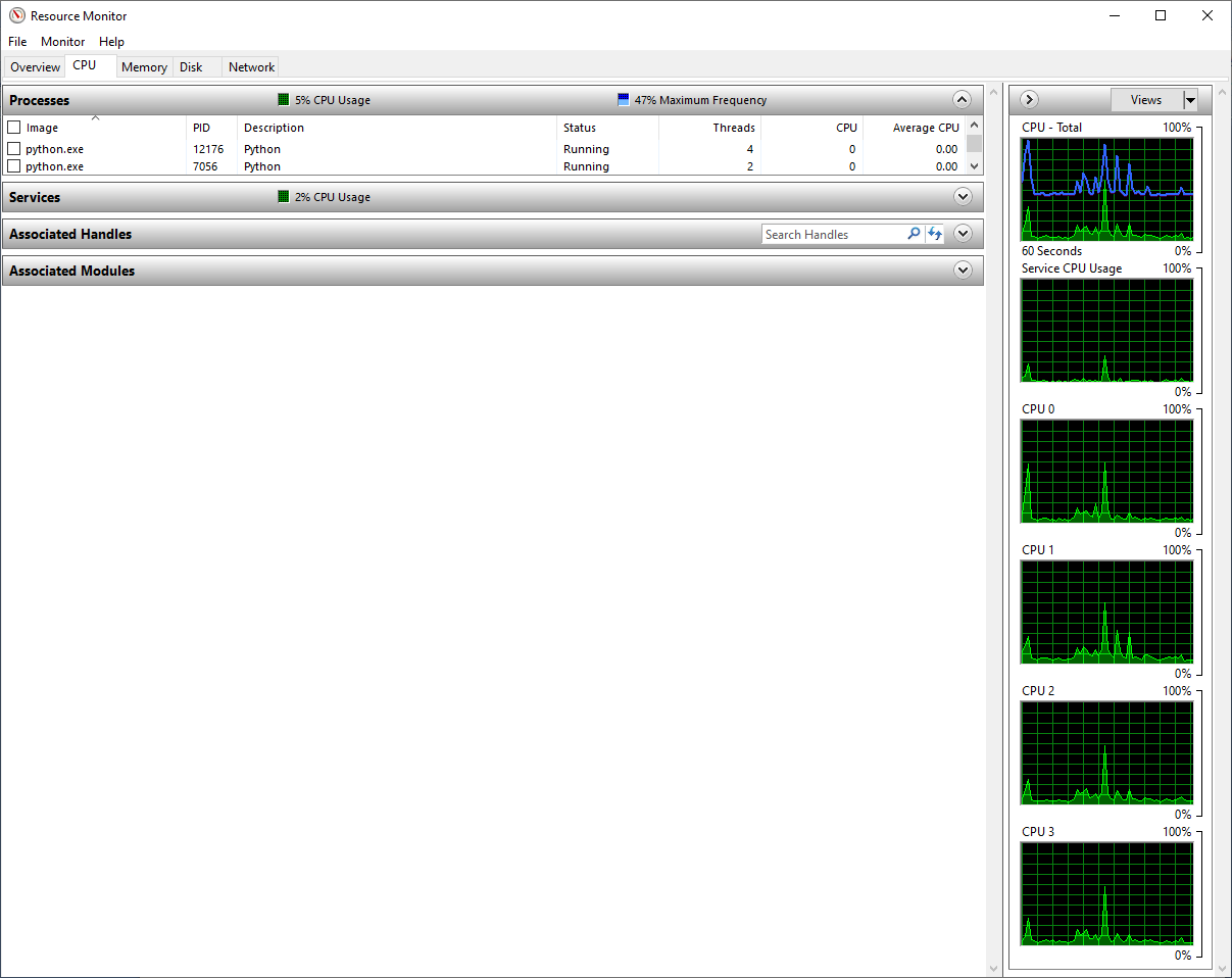
My machine has four CPU cores, and you can see these in the graphs on the right side labeled CPU 0, CPU 1, CPU 2, and CPU 3. You can see in the process list that I have two Python processes with a few threads allocated, but with nothing running, the CPU usage for my Python processes is effectively zero. In the rest of the tests in this article, I will be using Resource Monitor to track how Python runs my code on my machine. Note, if you use Visual Studio Code on a Macintosh, this tool may be helpful. If you run Linux, "htop" or a related tool may allow you to see the same information
Installation and Testing Notes (Same Setup as Previous Article)
I installed Python from the standard CPython site. I then used pip to install all the needed modules in the code below. All testing was performed locally on my personal PC running Windows 10. Python version was 3.8.1 (visible by typing “python –V” at the command prompt), SciPy version was 1.4.1, and NumPy version was 1.18.1 (access module versions by printing/examining <MODULE NAME>.__version__). I performed all testing using Visual Studio Code with the installed Python extension. Note, when debugging Python in Visual Studio Code (VS Code), once you have the Python extension installed, follow these instructions to setup your debugging configuration. This will create a launch.json file in your code directory. When you have that, if you want to be able to step into the module fitting (Numpy, SciPy, etc.), you need to add the justMyCode option and set it to false.
Simulate Test Data
Before we start writing code, we need to pause and look at how we can specifically test speed improvements on an NLLS Regression algorithm in Python? The nature of the fitting algorithms itself probably do not lend themselves to use multiprocessing, because of how these algorithms find a solution. Most NLLS Regression algorithms use Gradient Descent or something similar, which requires an initial starting position, then makes iterative calculations to descend to what it determines is the minimum. The position for what would be the next iteration is not known until the current iteration is complete, making this a serial/sequential algorithm - everything has to be processed in a specific order. Thus, we can't use parallel processing to speed up the NLLS Regression algorithm itself, and we will assume here that the creators of these algorithms have designed the inner workings to be as fast as possible. What we can run in parallel is this NLLS regression algorithm fitting on multiple sets of data. So, for this test, we will simulate repeated measurements from a singular phenomenon, so we can see how the parameters vary across a set of data. Like my previous article, we will use the same parametric mathematical model to generate and fit the data
y = exp(-β1∙x)∙cos(β2∙x) + ε
Now to generate the code, which can be found on my GitHub here. First, we need to import the required Python modules and their submodules/functions:
import numpy as np
from scipy.optimize import least_squares
import time
# Plotting module
import matplotlib.pyplot as plt
# Multiprocesing module
from multiprocessing import Pool
# Iteration tools module
from itertools import starmap
We are only going to use the Scipy NLLS Regression module least_squares in this test, which I discussed more in my previous article. We will use the model equation above to generate our noise-free "signal" data
def fcn2minExpCos(x, beta1, beta2):
    return np.exp(-beta1*x) * np.cos(beta2*x)
The next section of code is used to create the initial noise-free signal, starting with 101 values of our independent variable x, and the initial noise-free signal yNoiseFree. We then determine how many noisy data samples we want to generate from this base signal, in this case 10,000. We then allocate memory for our noisy data (NoisyDataSamples) and generate random, normally-distributed noise for all data points (10,000 x 101 = 1,010,000 individual noise calculations). This may be a bit confusing since we have essentially a two-dimensional data set, so I will try to keep my terminology consistent. The "noise-free signal" (yNoiseFree) is the original signal of 101 data points before noise is added, a "noisy data sample" (yNoisyDataSamples[i]) represents the above noise-free signal with noise added to each of its 101 data points. We will then attempt to fit each of these 10,000 noisy data samples with the least_squares algorithm and compare the estimated parameters with the original Beta1 and Beta2 values of 0.5 and 5. Note, there is a section of commented out code if you want to plot a specific noisy data sample versus the noise-free signal data.
x = np.linspace(0, 10.0, num=101)
Beta1 = 0.5
Beta2 = 5
NumParams = 2
StdNoise = 0.1
yNoiseFree = fcn2minExpCos(x, Beta1, Beta2)

# Add normally distributed noise multiple times to create a set of noisy data
NumberOfNoisyDataSamples = 10000
NoisyDataSamples = np.zeros((NumberOfNoisyDataSamples, len(x)))
for i in range(0, NumberOfNoisyDataSamples):
    RandomNoiseSamples = np.random.normal(size=len(x), scale=StdNoise)
    NoisyDataSamples[i, :] = yNoiseFree + RandomNoiseSamples

# Optional code to plot the original signal and overlay noisy data to show the scale of the noise
# plt.plot(x, yNoiseFree, 'b')
# plt.plot(x, NoisyDataSamples[0,:], 'r') # 0 represents the first noisy data set
# plt.xlabel('x')
# plt.ylabel('yNoiseFree (blue) and NoisyDataSamples (red)')
# plt.show()
For Loop
Before we attempt to use the multiprocessing module, we will set our baseline to be calling the fitting algorithm on each of the 10,000 noisy data samples sequentially using a for loop. First declare our output parameter arrays as well as the initial parameter guess for the fitting algorithm outside of the loop
InitialParams = [1., 1.]
Beta1ParamArray = np.zeros(NumberOfNoisyDataSamples)
Beta2ParamArray = np.zeros(NumberOfNoisyDataSamples)
Now the for loop implementation of the least_squares fitting algorithm on all noisy data samples. Note, for this initial test we are not providing a specific calculation of the Jacobian, with the Jacobian-specific function call commented out. This will be examined later. Note, we are also using the lm or Levenberg-Marquart fitting algorithm option, and I have bounded the for loop with the time module functions to measure how long the enclosed code takes.
startFitting = time.time()
for i in range(0, NumberOfNoisyDataSamples):
    NoisyDataSet = NoisyDataSamples[i, :]
    # Option - fit without Jacobian
    LSOptimResult = least_squares(fcn2minExpCosErrFunc, InitialParams, method='lm', args=(x, NoisyDataSet), verbose=0)
    # Option - fit with Jacobian
    # LSOptimResult = least_squares(fcn2minExpCosErrFunc, InitialParams, jac=jac2minExpCosErrFunc, method='lm', args=(x, NoisyDataSet), verbose=0)
    Beta1ParamArray[i] = LSOptimResult.x[0]
    Beta2ParamArray[i] = LSOptimResult.x[1]

endFitting = time.time()
print('Total Fitting Time: ' + str(endFitting - startFitting))
And finally, the fitting function for the algorithm:
def fcn2minExpCosErrFunc(beta, x, y):
    return (y - (np.exp(-beta[0]*x) * np.cos(beta[1]*x)))
After running these options in the script, I found the total run time to fit all 10,000 data samples to take 22 - 23 seconds. To see how my machine runs this code, I took a snapshot of the Resource Monitor shortly after this script started running

In this image, you can see that a new Python process has spawned and it is consuming 25 percent of my CPU resources or 1 out of 4 cores. Interestingly, there is an increase of activity on the graphs of all four of my cores, suggesting that Windows is internally processing some of this code on multiple threads which can span multiple cores. However, we are still running on one-fourth of our computational capacity because the Python code itself is running on one core. Let's try and see if we can speed things up using the multiprocessing module.
Multiprocessing
Getting the multiprocess module working requires a little more work than the for loop method, and the Python documentation for this can be a bit daunting. After doing some testing and researching other folks’ solutions on the internet, I got this to work. First, you have to create a new, separate function, put the fitting function call inside this function, and return the values you want out.
def FitNoisyData(x, NoisyDataSet):
    # Option - fit without Jacobian
    LSOptimResult = least_squares(fcn2minExpCosErrFunc, InitialParams, method='lm', args=(x, NoisyDataSet), verbose=0)
    # Option - fit with Jacobian
    # LSOptimResult = least_squares(fcn2minExpCosErrFunc, InitialParams, jac=jac2minExpCosErrFunc, method='lm', args=(x, NoisyDataSet), verbose=0)
    return [LSOptimResult.x[0], LSOptimResult.x[1]]
You then need to replicate the x-axis data (variable x) using the tile function, declare the Pool size to be the number of processes you want to use (in my case 4, since that’s how many cores my CPU has), interlace the x values and data together to create the dataset using the zip function, and finally call the pool starmap function to perform the function call FitNoisyData to the fitting algorithm.
# Add this line for Pool to work properly
if __name__ == '__main__':
    startFitting = time.time()
    # Tile the x values multiple times to match the data array size
    xTiled = np.tile(x, (NumberOfNoisyDataSamples, 1))
    # Setup multiprocessing pool
    pool = Pool(4)
    ResultList = pool.starmap(FitNoisyData, zip(xTiled, NoisyDataSamples)) # Use zip to interlace the x and y values
    pool.close()
    pool.join()
    # Data gets returned as a list, convert to array to reshape for the parameter arrays
    ResultArray = np.array(ResultList)
    Beta1PoolParamArray = ResultArray[:,0]
    Beta2PoolParamArray = ResultArray[:,1]

    endFitting = time.time()
    print('Total Fitting Time: ' + str(endFitting - startFitting))
After running this section of script to fit the noisy sample data multiple times, the average run time was around 4 - 5 seconds!! This is a speed up of around 5x, more than the number of cores we have on the machine. You can see why the speed happens by looking at the Python processes in Performance Monitor. When the script is running, there are now four Python processes running, each using about 25% of CPU capability.
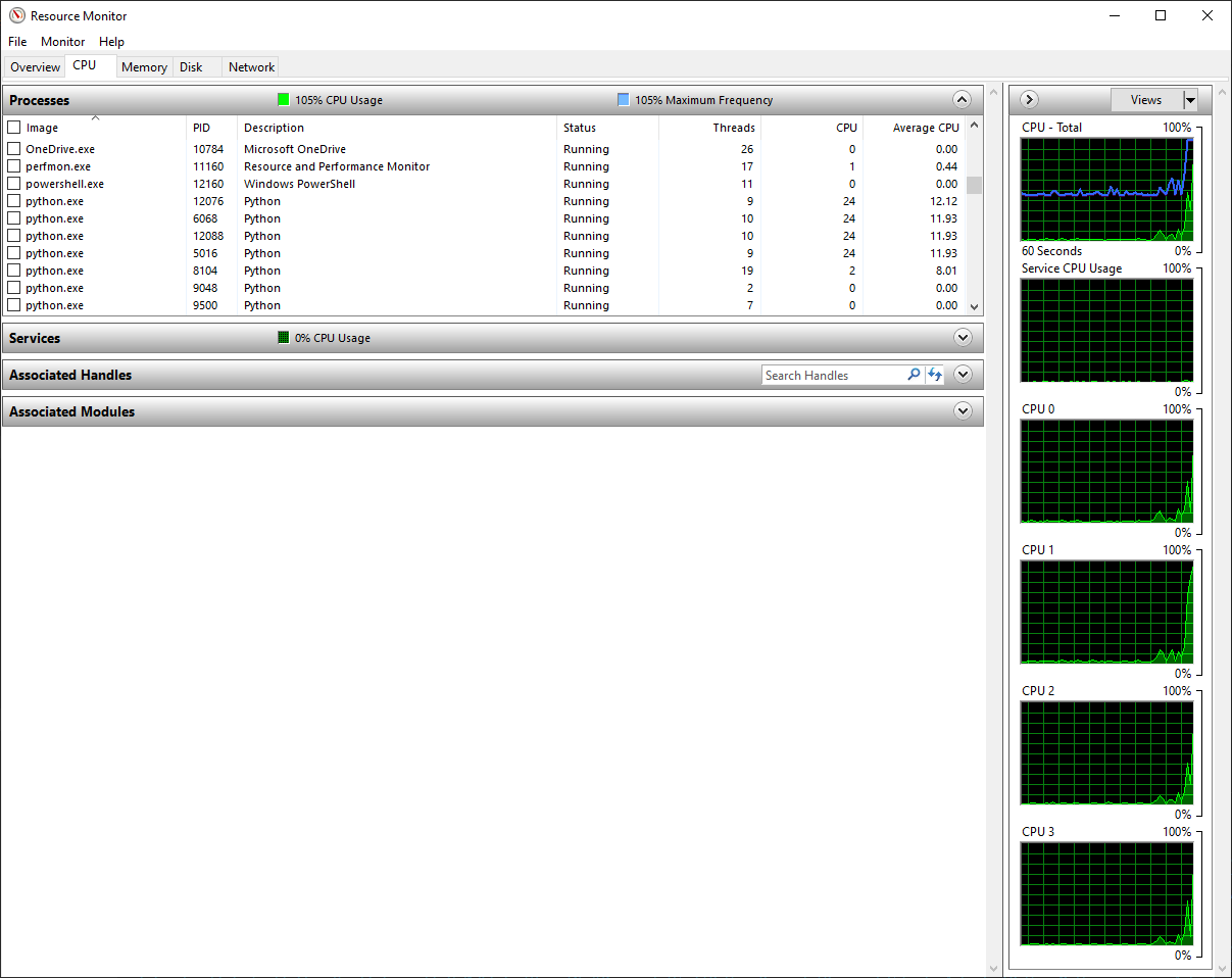
It’s hard to see in the CPU graphs, because the graphs lag a little bit behind and the script only runs for four seconds, but all four CPU cores are maxed out at 100% usage. Thus, the multiprocessing module is definitely a huge benefit here, since our run time is now less than 20% of the run time with the original for loop.
But wait - I'm in Debug Mode
After getting excited about the initial results of running with the multiprocessing module, something didn't sit quite right about getting a performance improvement more than the number of cores on the machine, so I went through all the possible ways that I could run this code and realized that my usual mode of running code in VS Code was to hit the F5 key, which runs in debug mode. Debug mode can extra time to the runtime of code since it can generate extra debug symbols so you can actually stop on lines of code, step to the next line of code, step into a function, etc. After running the for loop portion of my script several times (commenting out the multiprocessing code section), I was now getting run times of 10-11 seconds. My multiprocessing code was still consistently averaging run times around 4 seconds. So, while I'm still getting a good speed improvement using the multiprocessing code, my speed improvement factor is now only about 2.5x (40% of the runtime required versus for loop). This makes more sense once you take into account the overhead of the multiprocessing module setting up processes on other cores, delegating work to the other processes over the allowed methods, etc. To see whether this performance changes as the amount of data increases, I increased the number of data samples to fit on first to 50,000 and then to 100,000. After several tests with each method on these new increased data sets, here are the results I got:
for loop
50,000 data samples:
53-54 seconds
100,000 data samples:
107-108 seconds
multiprocessing
50,000 data samples:
16-17 seconds
100,000 data samples:
32-33 seconds
After the number of data was increased, we now see an increase in speed of around 3.25 - 3.5x improvement (code now runs in 30% of the time the for loop takes). This is more in the range that we would expect, closer a to 4x improvement (number of cores) minus some overhead. If our data set expanded to millions or billions of samples, we would expect the overhead to play even less of a part and we eventually hit some asymptotic limit close to 4x such that our code would run in 25% of the time that code without any parallel computing improvements would take.
A couple of notes
Some other tests that I did while running my code. One, I ran the script separately for both the for loop and multiprocessing configuration at the command line using "python Multiprocessing and Scipy NLLS Regression.py" to ensure that Visual Studio Code was not adding any additional overhead. These tests confirmed that the run times were similiar to running the script inside VS Code without the Debug option. Two, there are a lot of options for running multiple code in a method known as vectorization instead of inside a for/while loop. You will see some people report speed improvements out there using some methods. I tried this by using the Python itertools module and its starmap function (same format as the multiprocessing function)
# Python itertools starmap function
startFitting = time.time()
# Tile the x values multiple tiles to match the data
xTiled = np.tile(x, (NumberOfNoisyDataSamples, 1))
ResultList = list(starmap(FitNoisyData, zip(xTiled, NoisyDataSamples))) # Use zip to interlace the x and y values
ResultArray = np.array(ResultList)
Beta1ParamArray = ResultArray[:,0]
Beta2ParamArray = ResultArray[:,1]
endFitting = time.time()
print('Total Fitting Time: ' + str(endFitting - startFitting))
I found that I got similar run times to using the for loop. This may be due to the nature of the NLLS Regression algorithm running inside the mapping, since each individual regression algorithm function call has to run sequentially, as I discussed above. I would test whatever code you want to run inside a map/starmap yourself, and not take my results as a generalization. However, numpy does have a function called vectorize and in that documentation, they state that "The implementation is essentially a for loop". If you have to run a job on a machine that is non-multicore, options such as the ones found in itertools might prove fruitful.
MOAR SPEED - Providing an Explicit Jacobian
As I showed in my previous article, providing an explicitly-calculated Jacobian provided an additional reduction in fitting algorithm runtime. If I switched to the Jacobian-provided function calls in the for loop and multiprocessing code options above, and use the following Jacobian code:
def jac2minExpCosErrFunc(beta, x, y=None):
    # Model function =  np.exp(-beta1*x) * np.cos(beta2*x)
    JacobPt1 = -x * np.exp(-beta[0]*x) * np.cos(beta[1]*x) # d/da
    JacobPt2 = -x * np.exp(-beta[0]*x) * np.sin(beta[1]*x) # d/db
    return np.transpose([JacobPt1, JacobPt2])
I get the following run times for 100,000 data samples tested
for loop (no Jacobian)
107-108 sec
for loop (with Jacobian)
56-57 sec
multiprocessing (no Jacobian)
32-33 sec
multiprocessing (with Jacobian)
18-19 sec
Thus, it appears that for both methods, we get about a 2x speed improvement by explicitly providing a calculated Jacobian to the fitting algorithm. Providing both a Jacobian and using the multiprocessing module means our total run time was reduced from 107 seconds to 18 seconds, or about a 6x speed improvement (code would run in 17% of the time) over running a fit with no Jacobian in a for loop. So, if you have huge datasets that are taking you hours or days to run, even on a computing cluster, I hope this demonstration of using multiprocessing and explicitly providing a Jacobian will save you some time (and money) with your NLLS Regression fitting jobs.
Script
Again, this script is available on my GitHub repository here. I also uploaded it to my repl.it repository here. However, when testing it on repl.it, the performance of the multiprocessing was two times SLOWER than the standard for loop. I verified that there were also four cores on repl.it using the multiprocesssing cpu_count function. I am only on the Starter account, so it may be how repl.it is allocating computing resources virtually. Just a precaution, if you use repl.it consistently.